Basic Usage

As seen in the Quickstart guide, you can get going pretty quickly with an understanding of DataFrames.jl and Makie.jl. Let's walk through a couple of relatively simple examples.

Example 1 - setting up a basic plot

Info

Population bar chart

using GeoFacetMakie
using DataFrames
using Random

# Choose your preferred Makie backend:
using CairoMakie  # For static plots
CairoMakie.activate!()

# Set random seed for reproducible results
Random.seed!(42)

# Sample population data for US states
sample_data = DataFrame(
    state = [
        "CA", "TX", "NY", "FL", "WA", "PA", "IL", "OH", "GA", "NC",
        "MI", "NJ", "VA", "TN", "AZ", "MA", "IN", "MO", "MD", "WI",
    ],
    population = [
        39.5, 29.1, 19.8, 21.5, 7.6, 13.0, 12.7, 11.8, 10.7, 10.4,
        10.0, 9.3, 8.6, 6.9, 7.3, 7.0, 6.8, 6.2, 6.2, 5.9,
    ],
    gdp_per_capita = [
        75_277, 63_617, 75_131, 47_684, 71_362, 59_195, 65_886,
        54_021, 51_244, 54_578, 48_273, 70_034, 64_607, 52_375,
        45_675, 81_123, 54_181, 53_578, 65_641, 54_610,
    ],
    unemployment_rate = [
        4.2, 3.6, 4.3, 3.2, 4.6, 4.9, 4.2, 4.0, 3.1, 3.9,
        4.3, 4.1, 2.9, 3.3, 3.5, 2.9, 3.2, 2.8, 4.4, 3.2,
    ]
)

20×4 DataFrame

Row	state	population	gdp_per_capita	unemployment_rate
	String	Float64	Int64	Float64
1	CA	39.5	75277	4.2
2	TX	29.1	63617	3.6
3	NY	19.8	75131	4.3
4	FL	21.5	47684	3.2
5	WA	7.6	71362	4.6
6	PA	13.0	59195	4.9
7	IL	12.7	65886	4.2
8	OH	11.8	54021	4.0
9	GA	10.7	51244	3.1
10	NC	10.4	54578	3.9
11	MI	10.0	48273	4.3
12	NJ	9.3	70034	4.1
13	VA	8.6	64607	2.9
14	TN	6.9	52375	3.3
15	AZ	7.3	45675	3.5
16	MA	7.0	81123	2.9
17	IN	6.8	54181	3.2
18	MO	6.2	53578	2.8
19	MD	6.2	65641	4.4
20	WI	5.9	54610	3.2

When creating the plotting function, you need to create a mutating version. You may want to create a wrapper that creates the figure and then passes it to your mutating version, to confirm that everything plots as you intend with a test subset of the data.

function barplot_fn!(
    gl,
    data;
    missing_regions, # It's important to have this kwarg
    color = :steelblue,
    axis_kwargs...
)
    ax = Axis(
        gl[1, 1];
        title = data.state[1],
        axis_kwargs...
    )
    barplot!(ax, [1], data.population, color = color)
    return nothing
end

function barplot_fn(
    data;
    missing_regions = :skip,
    color = :steelblue,
    axis_kwargs...
)
    fig = Figure()
    gl = fig[1, 1] = GridLayout()
    barplot_fn!(
        gl,
        data;
        color = color,
        missing_regions = missing_regions,
        axis_kwargs...
    )
    return fig
end

barplot_fn (generic function with 1 method)

Let's show how we can pass some of the axis kwargs through to the Axis method call. If you would like any specific kwargs to be handled within the plotting function body, make sure to explicitly list them in the function signature, for example, color = :steelblue. This is because all other kwargs passed to the user function should be splat within the axis constructor.

fig_barplot = barplot_fn(
    subset(sample_data, :state => s -> s .== "CA");
    color = :red,
    xlabelvisible = false,
    xticksvisible = false,
    xticklabelsvisible = false,
    ylabel = "Population (M)",
    limits = (nothing, (0, 60))
)
fig_barplot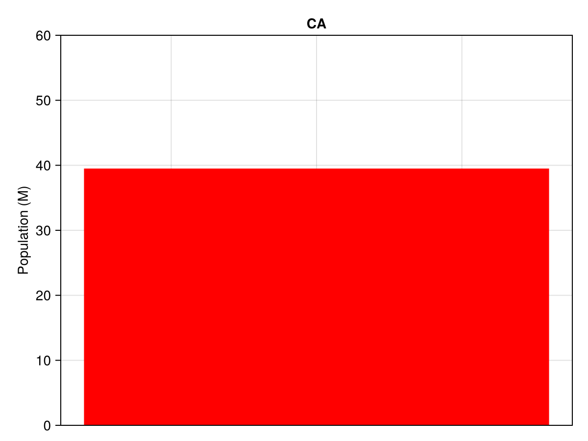

# Now works with new API
fig_barplot_geofacet = geofacet(
    sample_data,
    :state,
    barplot_fn!;
    link_axes = :both,
    figure_kwargs = (size = (1200, 800),),
    common_axis_kwargs = (
        titlesize = 14,
        ylabel = "Population (M)",
        xlabelvisible = false,
        xticksvisible = false,
        xticklabelsvisible = false,
        limits = (nothing, (0, 60))
    ),
    func_kwargs = ( # pass kwargs to the plotting function here
        missing_regions = :skip,
        color = :coral,
    )
)
fig_barplot_geofacet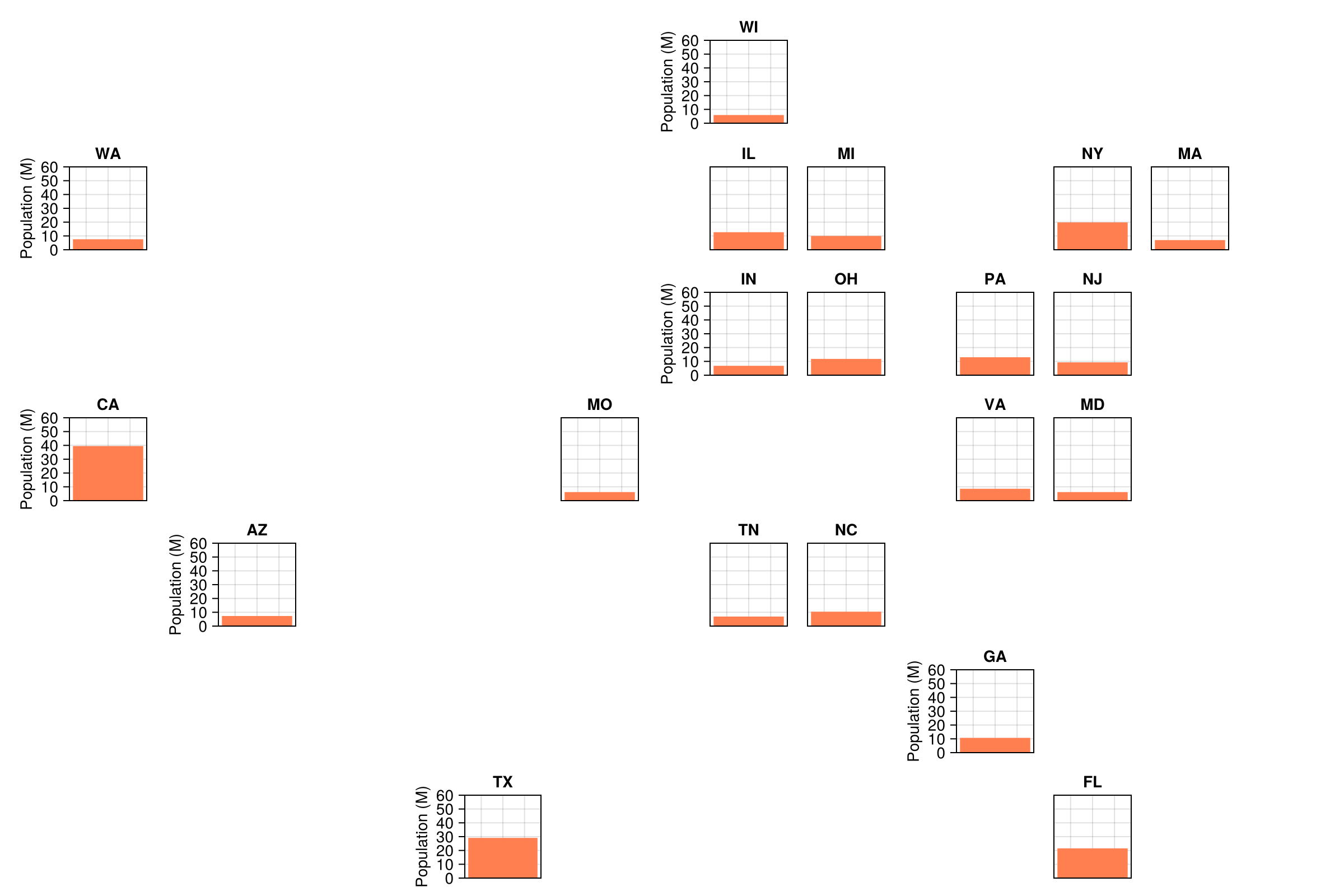

Example 2 - linking axes

Info

GDP vs Unemployment

Note

It is also possible to specify the plotting function with an anonymous function

Now let's link axes on a scatter plot. Because we are dealing with larger numbers, to make the x axis tick labels clearer, let's add some rotation. We'll also set the geofacet() kwarg hide_inner_decorations = false to plot all axis ticks and labels on each facet, not just those without a neighbor.

fig_linked_axes_geofacet = geofacet(
    sample_data, :state,
    (gl, data; missing_regions, axis_kwargs...) -> begin
        ax = Axis(gl[1, 1]; axis_kwargs...)
        scatter!(
            ax, data.gdp_per_capita, data.unemployment_rate,
            color = :coral, markersize = 12
        )
        ax.title = data.state[1]
    end,
    link_axes = :both,  # Link both x and y axes
    figure_kwargs = (size = (1800, 1200),),
    common_axis_kwargs = (
        xlabel = "GDP per capita (\$)",
        ylabel = "Unemployment (%)",
        xticklabelrotation = pi / 4,
    ),
    hide_inner_decorations = false
)
fig_linked_axes_geofacet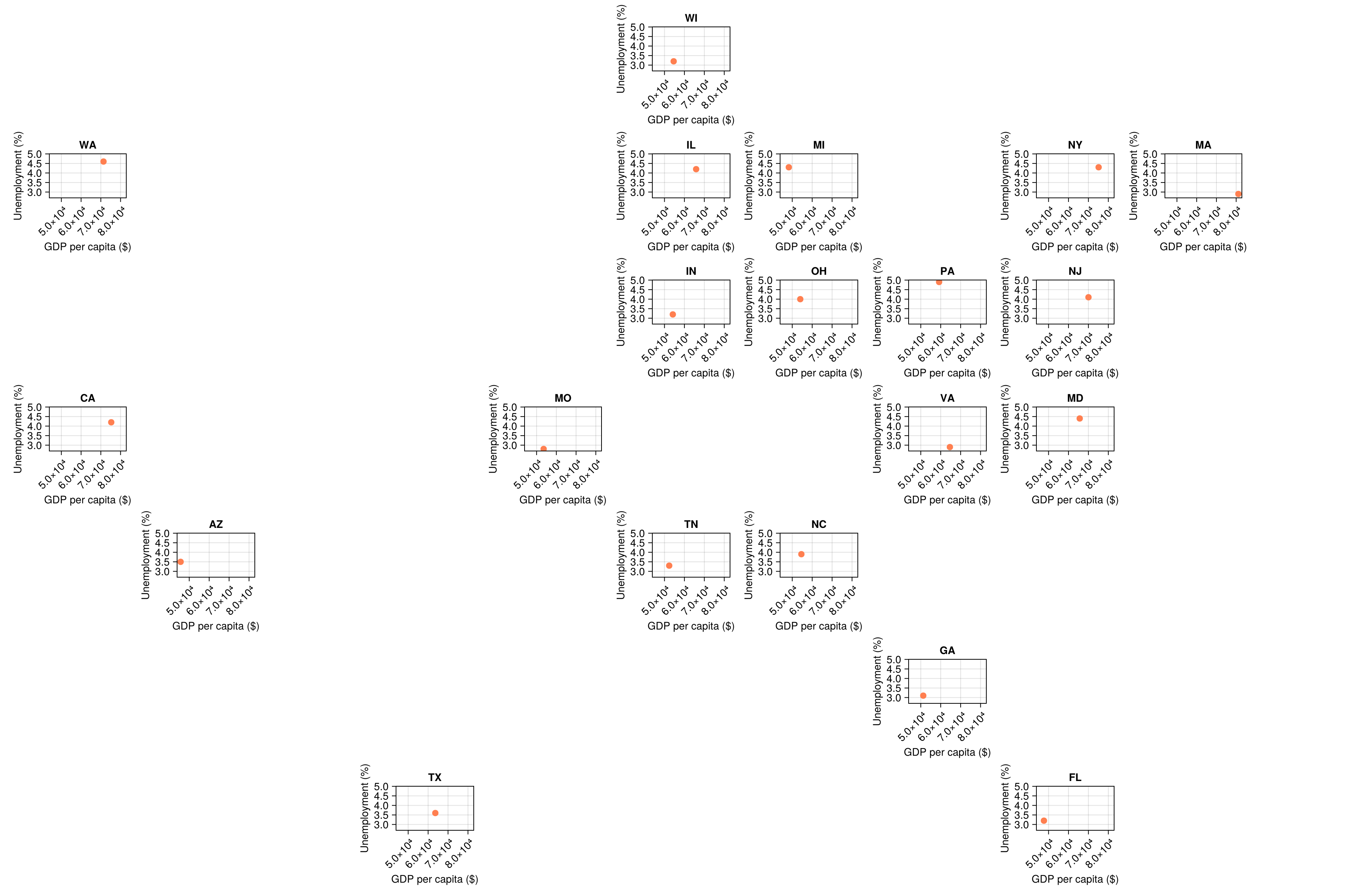

Example 3 - time series

Info

Population growth time series, and plot all facets, regardless of whether they contain time series data

# Create time series data
years = 2010:2023
all_state_data = DataFrame[]

for state in sample_data.state[1:10]  # Use first 10 states for cleaner demo
    base_pop = sample_data[sample_data.state .== state, :population][1]
    growth_rate = 0.005 + 0.01 * rand()  # Random growth rate between 0.5% and 1.5%

    state_data = DataFrame(
        state = fill(state, length(years)),
        year = collect(years),
        population = [base_pop * (1 + growth_rate)^(y - 2023) for y in years]
    )

    # Add this state's data to our collection
    push!(all_state_data, state_data)
end

time_series_data = vcat(all_state_data...)
first(time_series_data, 10)

10×3 DataFrame

Row	state	year	population
	String	Int64	Float64
1	CA	2010	34.1345
2	CA	2011	34.52
3	CA	2012	34.9098
4	CA	2013	35.3041
5	CA	2014	35.7028
6	CA	2015	36.106
7	CA	2016	36.5138
8	CA	2017	36.9261
9	CA	2018	37.3432
10	CA	2019	37.7649

fig_time_series_geofacet = geofacet(
    time_series_data, :state,
    (gl, data; missing_regions, axis_kwargs...) -> begin
        ax = Axis(gl[1, 1]; axis_kwargs...)
        lines!(
            ax, data.year, data.population,
            color = :darkgreen, linewidth = 2
        )
        ax.title = data.state[1]
    end,
    link_axes = :both,  # Link both x- and y-axes for comparison
    figure_kwargs = (size = (1200, 800),),
    common_axis_kwargs = (
        titlesize = 14,
        xlabel = "Year",
        ylabel = "Population (M)",
        xlabelsize = 12,
        ylabelsize = 12,
        xticklabelsize = 10,
        yticklabelsize = 10,
    ),
    func_kwargs = (missing_regions = :empty,)
)
fig_time_series_geofacet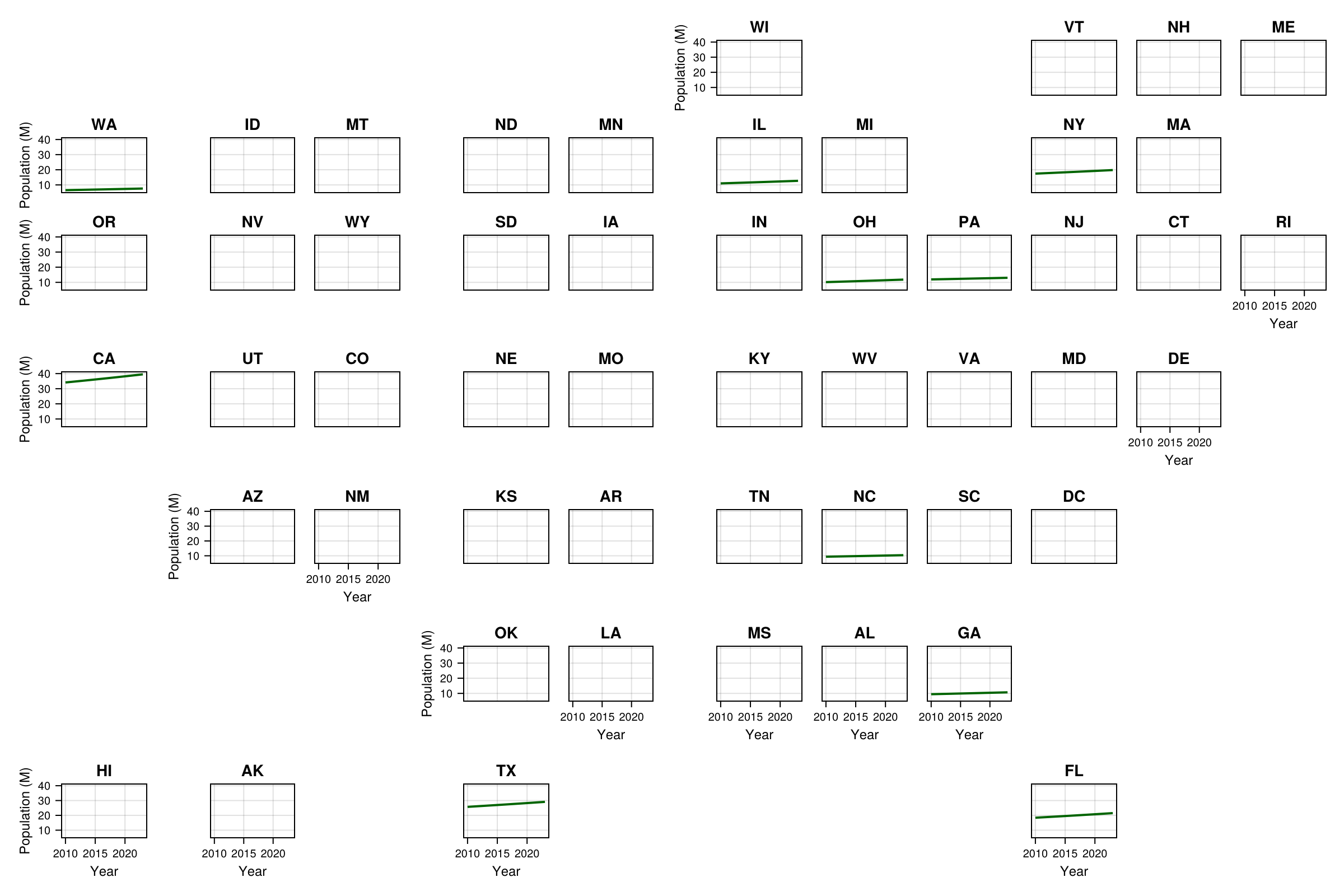

Example 4 - regions that don't exist in the grid

If your data contains region codes that don't exist in the grid, you should receive an error, unless you set the additional_regions kwarg equal to :warn.

julia> # Create data with some states that don't exist in the grid
       error_data = DataFrame(
           state = ["CA", "TX", "INVALID", "FAKE_STATE", "NY"],
           value = [1, 2, 3, 4, 5]
       )
5×2 DataFrame
 Row │ state       value 
     │ String      Int64 
─────┼───────────────────
   1 │ CA              1
   2 │ TX              2
   3 │ INVALID         3
   4 │ FAKE_STATE      4
   5 │ NY              5

julia> fig_additional_regions_geofacet = geofacet( # this errors
           error_data, :state,
           (gl, data; missing_regions, axis_kwargs...) -> begin
               ax = Axis(gl[1, 1]; axis_kwargs...)
               barplot!(ax, [1], data.value, color = :orange)
               ax.title = data.state[1]
           end;
           additional_regions = :error
       )
ERROR: ArgumentError: Additional regions in data not present in the grid provided: INVALID, FAKE_STATE

julia> fig_additional_regions_geofacet = geofacet( # This warns and continues
           error_data, :state,
           (gl, data; missing_regions, axis_kwargs...) -> begin
               ax = Axis(gl[1, 1]; axis_kwargs...)
               barplot!(ax, [1], data.value, color = :orange)
               ax.title = data.state[1]
           end;
           additional_regions = :warn
       )
┌ Warning: Additional regions in data not present in the grid provided: INVALID, FAKE_STATE
└ @ GeoFacetMakie ~/work/GeoFacetMakie.jl/GeoFacetMakie.jl/src/plotting/geofacet_core.jl:103
Figure()

fig_additional_regions_geofacet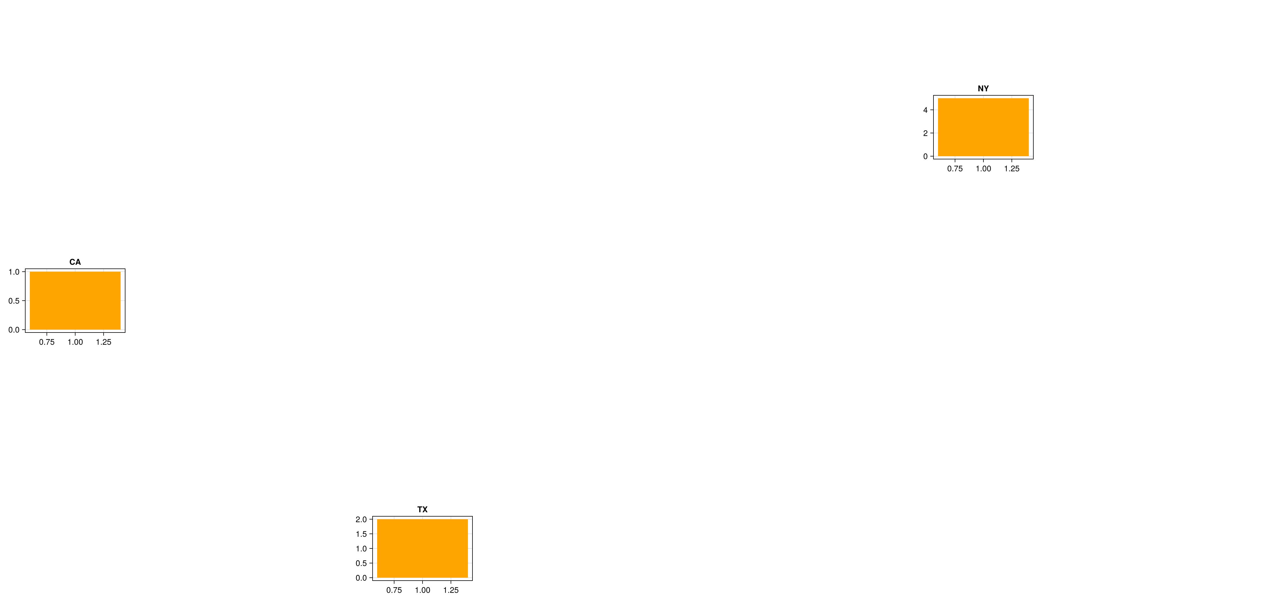

Example 5 - forgetting missing_regions

Your user function should accept the missing_regions kwarg (as well as handle it). If you do not specify it then you should receive an error warning you to rectify this. This is because the user function must provide the confirmation whether the necessary data for the plot exists and error if missing_regions is set to :error.

julia> geofacet(
           time_series_data, :state,
           (gl, data; axis_kwargs...) -> begin
               ax = Axis(gl[1, 1]; axis_kwargs...)
               lines!(
                   ax, data.year, data.population,
                   color = :darkgreen, linewidth = 2
               )
               ax.title = data.state[1]
           end,
           link_axes = :y,  # Link y-axes for comparison
           figure_kwargs = (size = (1200, 800),),
           common_axis_kwargs = (
               titlesize = 14,
               xlabel = "Year",
               ylabel = "Population (M)",
               xlabelsize = 12,
               ylabelsize = 12,
               xticklabelsize = 10,
               yticklabelsize = 10,
           ),
           func_kwargs = (missing_regions = :empty,)
       )
ERROR: Make sure to include `missing_regions` as a kwarg in your plotting function definition!