More Advanced Usage

Let's walk through a more involved example where we have multiple axes within a given facet.

Setting up the data

julia

using GeoFacetMakie
using DataFrames
using Random

# Choose your preferred Makie backend:
using CairoMakie  # For static plots

# Set random seed for reproducible results
Random.seed!(123)

# All 50 states + DC with 2023 baseline data
state_info = DataFrame(
    state = [
        "AL", "AK", "AZ", "AR", "CA", "CO", "CT", "DC", "DE", "FL", "GA",
        "HI", "ID", "IL", "IN", "IA", "KS", "KY", "LA", "ME", "MD",
        "MA", "MI", "MN", "MS", "MO", "MT", "NE", "NV", "NH", "NJ",
        "NM", "NY", "NC", "ND", "OH", "OK", "OR", "PA", "RI", "SC",
        "SD", "TN", "TX", "UT", "VT", "VA", "WA", "WV", "WI", "WY"
    ],
    population_2023 = [
        5.2, 0.73, 7.4, 3.0, 39.0, 5.8, 3.6, 1.5, 1.0, 22.6, 11.0,
        1.4, 1.9, 12.6, 6.8, 3.2, 2.9, 4.5, 4.6, 1.4, 6.2,
        7.0, 10.0, 5.7, 2.9, 6.2, 1.1, 2.0, 3.2, 1.4, 9.3,
        2.1, 19.3, 10.7, 0.78, 11.8, 4.0, 4.2, 13.0, 1.1, 5.3,
        0.91, 7.0, 30.0, 3.4, 0.65, 8.7, 7.8, 1.8, 5.9, 0.58
    ],
    gdp_per_capita_2023 = [
        49_861, 77_477, 55_313, 49_475, 89_540, 80_184, 90_213, 75_192, 85_939, 57_703, 58_608,
        65_393, 52_225, 78_291, 60_780, 65_555, 59_917, 52_295, 51_073, 56_277, 75_847,
        95_029, 55_675, 71_715, 40_464, 57_290, 54_506, 66_661, 64_296, 77_933, 75_715,
        49_754, 95_043, 60_592, 88_865, 65_278, 51_424, 71_342, 70_979, 64_340, 54_672,
        61_346, 58_492, 73_092, 68_758, 54_166, 74_222, 86_265, 47_529, 63_293, 75_648
    ]
)

first(state_info, 10)

10×3 DataFrame

Row	state	population_2023	gdp_per_capita_2023
	String	Float64	Int64
1	AL	5.2	49861
2	AK	0.73	77477
3	AZ	7.4	55313
4	AR	3.0	49475
5	CA	39.0	89540
6	CO	5.8	80184
7	CT	3.6	90213
8	DC	1.5	75192
9	DE	1.0	85939
10	FL	22.6	57703

julia

years = 2009:2023
# Create array to collect all state DataFrames
all_state_data = DataFrame[]

for row in eachrow(state_info)
    state = row.state
    base_pop = row.population_2023
    base_gdp = row.gdp_per_capita_2023

    # Generate realistic growth patterns
    pop_growth_rate = 0.003 + 0.015 * rand()  # 0.3% to 1.8% annual growth
    gdp_growth_rate = 0.01 + 0.03 * rand()    # 1% to 4% annual growth

    # Add some economic volatility (2008 crisis, COVID impact)
    pop_volatility = 0.002 * randn(length(years))
    gdp_volatility = 0.05 * randn(length(years))

    # Special adjustments for economic events
    crisis_years = [2009, 2010]  # Financial crisis
    covid_years = [2020, 2021]   # COVID impact

    # Pre-allocate arrays for this state's data
    state_populations = Float64[]
    state_gdps = Float64[]

    for (i, year) in enumerate(years)
        # Calculate years back from 2023
        years_back = 2023 - year

        # Base growth calculation
        pop_factor = (1 + pop_growth_rate)^(-years_back)
        gdp_factor = (1 + gdp_growth_rate)^(-years_back)

        # Apply volatility
        pop_vol = pop_volatility[i]
        gdp_vol = gdp_volatility[i]

        # Economic crisis adjustments
        if year in crisis_years
            gdp_vol -= 0.08  # GDP hit during financial crisis
            pop_vol -= 0.005  # Slower population growth
        elseif year in covid_years
            gdp_vol -= 0.05  # COVID economic impact
            pop_vol -= 0.003  # COVID population impact
        end

        # Calculate final values
        population = base_pop * pop_factor * (1 + pop_vol)
        gdp_per_capita = base_gdp * gdp_factor * (1 + gdp_vol)

        push!(state_populations, max(0.1, population))  # Ensure positive
        push!(state_gdps, max(20000, gdp_per_capita))  # Ensure reasonable minimum
    end

    # Create DataFrame for this state with all data at once
    state_data = DataFrame(
        state = fill(state, length(years)),
        year = collect(years),
        population = state_populations,
        gdp_per_capita = state_gdps
    )

    # Add this state's data to our collection
    push!(all_state_data, state_data)
end

# Combine all state data into one DataFrame
time_series_data = vcat(all_state_data...)

first(time_series_data, 10)

10×4 DataFrame

Row	state	year	population	gdp_per_capita
	String	Int64	Float64	Float64
1	AL	2009	4.44057	31386.6
2	AL	2010	4.49482	32603.3
3	AL	2011	4.57274	33687.4
4	AL	2012	4.62167	34782.4
5	AL	2013	4.66559	37712.6
6	AL	2014	4.70724	37482.0
7	AL	2015	4.77051	43963.4
8	AL	2016	4.82343	42604.0
9	AL	2017	4.87629	41232.5
10	AL	2018	4.92909	45691.5

Creating the plotting function

julia

"""
    dual_timeseries_plot!(gl, data; processed_axis_kwargs_list)

Mutating plotting function that creates dual time series plots using the new multi-axis API:
- Population (left y-axis, blue line)
- GDP per capita (right y-axis, red line)

This function demonstrates the new multi-axis kwargs API where each axis receives
its own processed kwargs from the geofacet function.
"""
function dual_timeseries_plot!(gl, data; missing_regions = :empty, processed_axis_kwargs_list)
    # Ensure data is sorted by year
    sorted_data = sort(data, :year)

    # Create population axis with first set of processed kwargs
    pop_ax = Axis(gl[1, 1]; processed_axis_kwargs_list[1]...)

    # Create GDP axis with second set of processed kwargs
    gdp_ax = Axis(gl[1, 1]; processed_axis_kwargs_list[2]...)

    # Plot population on primary y-axis (left)
    lines!(
        pop_ax,
        sorted_data.year,
        sorted_data.population,
        color = :steelblue,
        linewidth = 2.5,
    )

    # Configure primary axis (population)
    pop_ax.title = sorted_data.state[1]

    # Configure secondary axis (GDP) - styling applied via kwargs
    # Additional styling not covered by kwargs

    # Plot GDP on secondary y-axis (right)
    lines!(
        gdp_ax,
        sorted_data.year,
        sorted_data.gdp_per_capita,
        color = :firebrick,
        linewidth = 2.5,
    )

    return nothing
end

Main.dual_timeseries_plot!

Testing the plot

julia

ca_data = subset(time_series_data, :state => s -> s .== "CA")
test_fig = Figure(size = (400, 300))
test_gl = test_fig[1, 1] = GridLayout()

# Create test kwargs list for the new API
test_kwargs_list = [
	# Population Axis
    (
    	xlabel = "Year",
    	ylabel = "Population (M)",
    	titlesize = 12,
    	ylabelcolor = :steelblue,
    	yticklabelcolor = :steelblue,

    ),
	# GDP Axis
    (
    	yaxisposition = :right,
    	ylabel = "GDP per capita (\$)",
    	ylabelcolor = :firebrick,
    	yticklabelcolor = :firebrick,
		# Don't want duplication of axis and grid, so disable
		xticksvisible = false,
		xticklabelsvisible = false,
		xgridvisible = false,
		ygridvisible = false,
		leftspinevisible = false,
		rightspinevisible = false,
		bottomspinevisible = false,
		topspinevisible = false,
    )
]
dual_timeseries_plot!(test_gl, ca_data; processed_axis_kwargs_list = test_kwargs_list)
test_fig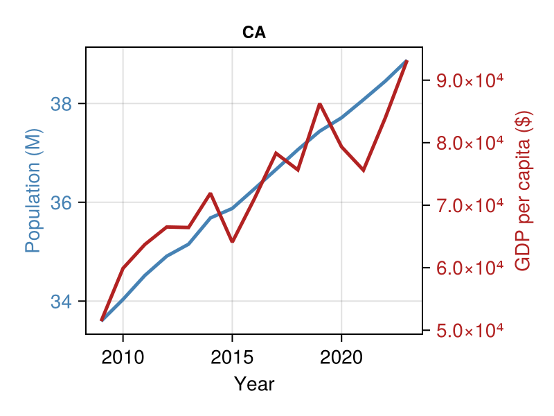

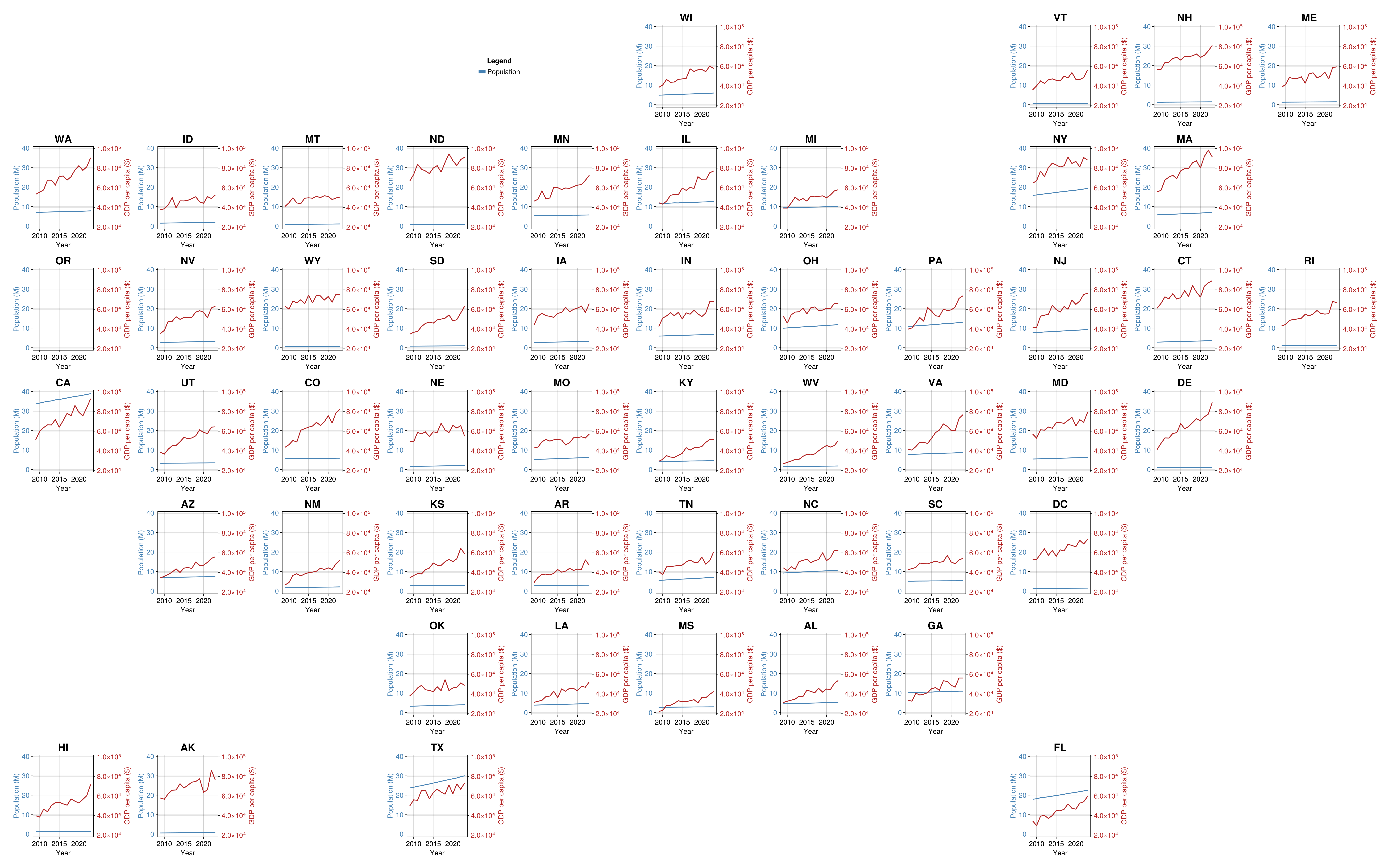
Geofacet

julia

geofacet(
	# Remove OR to confirm that empty states are handled correctly on both axes
	subset(time_series_data, :state => s -> s .!= "OR"),
    :state,
    dual_timeseries_plot!;  # Pass our named function
    figure_kwargs = (size = (4000, 2500), fontsize = 20),
    common_axis_kwargs = (
        titlesize = 30,
    ),
    axis_kwargs_list = [
        # Population axis (left)
        (xlabel = "Year", ylabel = "Population (M)",
         ylabelcolor = :steelblue, yticklabelcolor = :steelblue),
        # GDP axis (right)
        (yaxisposition = :right, ylabel = "GDP per capita (\$)",
         ylabelcolor = :firebrick, yticklabelcolor = :firebrick)
    ],
    link_axes = :both,  # Link x- and y-axes for comparison across time and space
    func_kwargs = (missing_regions = :empty, ),
    hide_inner_decorations = false # don't hide decorations for easier value checks
)

Adding a legend

To add a legend, you need to label the data in your plotting function. Let's update it accordingly.

julia

function dual_timeseries_plot!(gl, data; missing_regions = :empty, processed_axis_kwargs_list)
    # Ensure data is sorted by year
    sorted_data = sort(data, :year)

    # Create population axis with first set of processed kwargs
    pop_ax = Axis(gl[1, 1]; processed_axis_kwargs_list[1]...)

    # Create GDP axis with second set of processed kwargs
    gdp_ax = Axis(gl[1, 1]; processed_axis_kwargs_list[2]...)

    # Plot population on primary y-axis (left)
    lines!(
        pop_ax,
        sorted_data.year,
        sorted_data.population,
        color = :steelblue,
        linewidth = 2.5,
        label = "Population"
    )

    # Configure primary axis (population)
    pop_ax.title = sorted_data.state[1]

    # Configure secondary axis (GDP) - styling applied via kwargs
    # Additional styling not covered by kwargs

    # Plot GDP on secondary y-axis (right)
    lines!(
        gdp_ax,
        sorted_data.year,
        sorted_data.gdp_per_capita,
        color = :firebrick,
        linewidth = 2.5,
        label = "GDP per capita"
    )

    return nothing
end

dual_timeseries_plot! (generic function with 1 method)

julia

geofacet(
	# Remove OR to confirm that empty states are handled correctly on both axes
	subset(time_series_data, :state => s -> s .!= "OR"),
    :state,
    dual_timeseries_plot!;  # Pass our named function
    figure_kwargs = (size = (4000, 2500), fontsize = 20),
    common_axis_kwargs = (
        titlesize = 30,
    ),
    axis_kwargs_list = [
        # Population axis (left)
        (xlabel = "Year", ylabel = "Population (M)",
         ylabelcolor = :steelblue, yticklabelcolor = :steelblue),
        # GDP axis (right)
        (yaxisposition = :right, ylabel = "GDP per capita (\$)",
         ylabelcolor = :firebrick, yticklabelcolor = :firebrick)
    ],
    link_axes = :both,  # Link x- and y-axes for comparison across time and space
    func_kwargs = (missing_regions = :empty, ),
    hide_inner_decorations = false, # don't hide decorations for easier value checks
    legend_kwargs = (title = "Legend", framevisible = false)
)

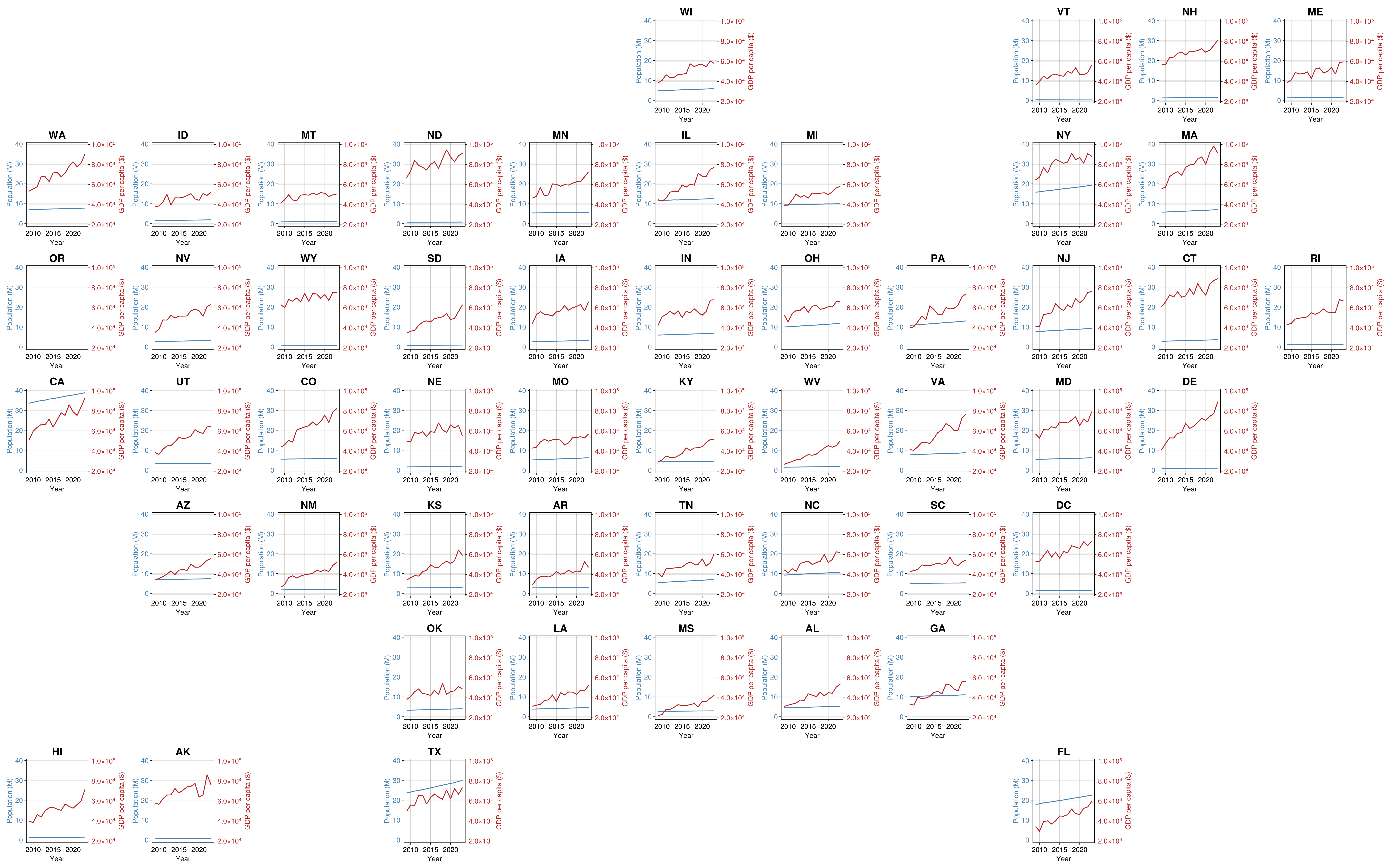
Updating the legend position

By default, the legend will be added to the right of the geofacet plot. If, however, you have a spare cell that you would like it to be placed at, use the legend_position = (row, column) specification within legend_kwargs. This can include a range if you would like the legend to span multiple GridLayouts.

julia

geofacet(
	# Remove OR to confirm that empty states are handled correctly on both axes
	subset(time_series_data, :state => s -> s .!= "OR"),
    :state,
    dual_timeseries_plot!;  # Pass our named function
    figure_kwargs = (size = (4000, 2500), fontsize = 20),
    common_axis_kwargs = (
        titlesize = 30,
    ),
    axis_kwargs_list = [
        # Population axis (left)
        (xlabel = "Year", ylabel = "Population (M)",
         ylabelcolor = :steelblue, yticklabelcolor = :steelblue),
        # GDP axis (right)
        (yaxisposition = :right, ylabel = "GDP per capita (\$)",
         ylabelcolor = :firebrick, yticklabelcolor = :firebrick)
    ],
    link_axes = :both,  # Link x- and y-axes for comparison across time and space
    func_kwargs = (missing_regions = :empty, ),
    hide_inner_decorations = false, # don't hide decorations for easier value checks
    legend_kwargs = (
        title = "Legend",
        framevisible = false,
        legend_position = (1, 4:5)
    )
)

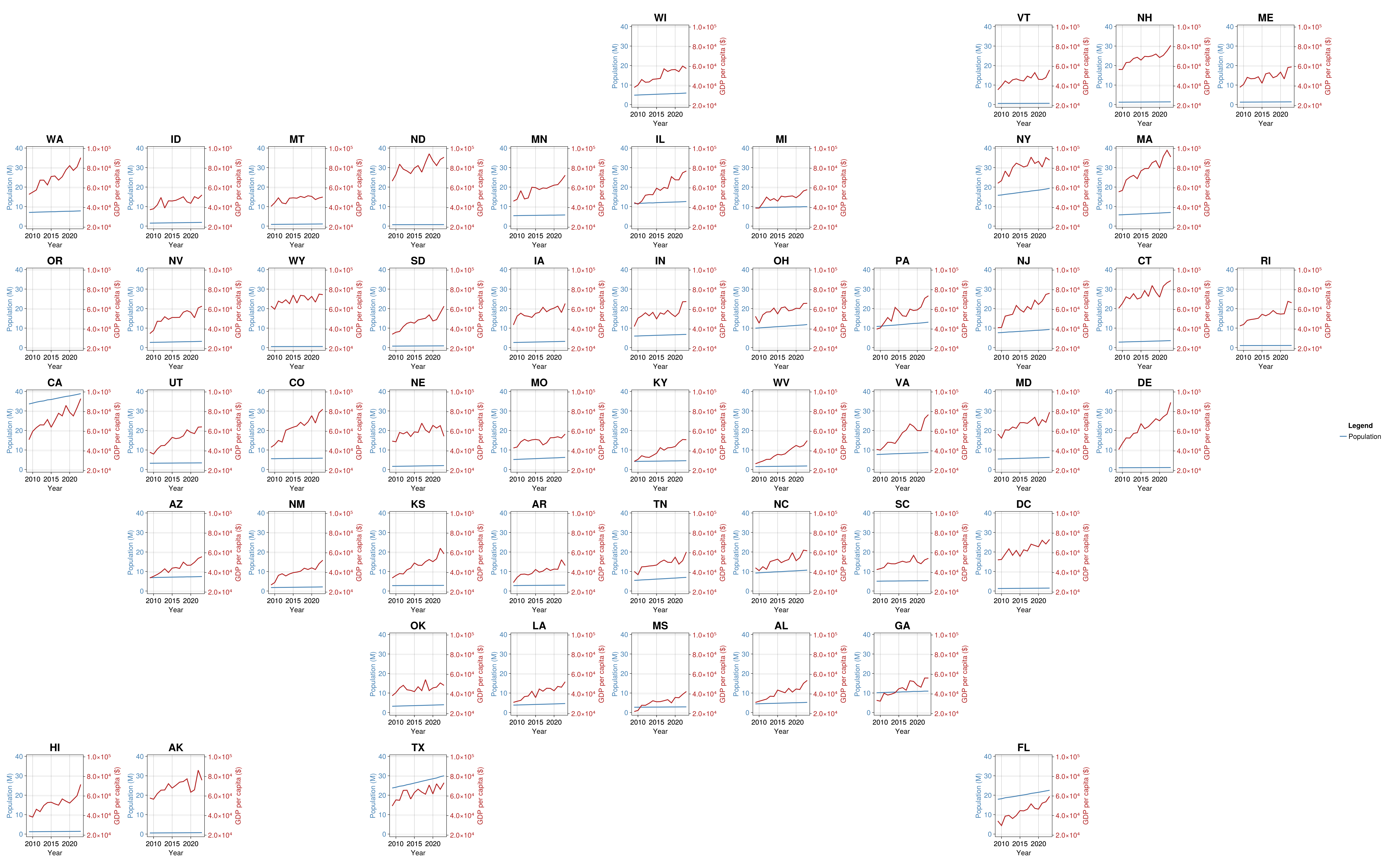
Updating the legend characteristics

If you would like to modify certain characteristics of the legend e.g., the markersize or linewidth, you can do this by modifying your plotting function as below.

julia

function dual_timeseries_plot!(
    gl,
    data;
    missing_regions = :empty,
    linewidth = 2.5,
    legend_linewidth = 2.5,
    processed_axis_kwargs_list
)
    # Ensure data is sorted by year
    sorted_data = sort(data, :year)

    # Create population axis with first set of processed kwargs
    pop_ax = Axis(gl[1, 1]; processed_axis_kwargs_list[1]...)

    # Create GDP axis with second set of processed kwargs
    gdp_ax = Axis(gl[1, 1]; processed_axis_kwargs_list[2]...)

    # Plot population on primary y-axis (left)
    lines!(
        pop_ax,
        sorted_data.year,
        sorted_data.population,
        color = :steelblue,
        linewidth = linewidth,
        label = "Population" => (; linewidth = legend_linewidth),

    )

    # Configure primary axis (population)
    pop_ax.title = sorted_data.state[1]

    # Configure secondary axis (GDP) - styling applied via kwargs
    # Additional styling not covered by kwargs

    # Plot GDP on secondary y-axis (right)
    lines!(
        gdp_ax,
        sorted_data.year,
        sorted_data.gdp_per_capita,
        color = :firebrick,
        linewidth = linewidth,
        label = "GDP per capita" => (; linewidth = legend_linewidth),
    )

    return nothing
end

dual_timeseries_plot! (generic function with 1 method)

Important

Because you have modified your plotting function, the variable has to be passed to func_kwargs, NOT legend_kwargs. This is because legend_kwargs constructs your Legend outside of your plotting function after the Axis and GridLayout has already been created.

julia

geofacet(
	# Remove OR to confirm that empty states are handled correctly on both axes
	subset(time_series_data, :state => s -> s .!= "OR"),
    :state,
    dual_timeseries_plot!;  # Pass our named function
    figure_kwargs = (size = (4000, 2500), fontsize = 20),
    common_axis_kwargs = (
        titlesize = 30,
    ),
    axis_kwargs_list = [
        # Population axis (left)
        (xlabel = "Year", ylabel = "Population (M)",
         ylabelcolor = :steelblue, yticklabelcolor = :steelblue),
        # GDP axis (right)
        (yaxisposition = :right, ylabel = "GDP per capita (\$)",
         ylabelcolor = :firebrick, yticklabelcolor = :firebrick)
    ],
    link_axes = :both,  # Link x- and y-axes for comparison across time and space
    func_kwargs = (
        missing_regions = :empty,
        legend_linewidth = 10,
    ),
    hide_inner_decorations = false, # don't hide decorations for easier value checks
    legend_kwargs = (
        title = "Legend",
        framevisible = false,
        legend_position = (1, 4:5),
    )
)

More Advanced Usage ​

Setting up the data ​

Creating the plotting function ​

Testing the plot ​

Geofacet ​

Adding a legend ​

Updating the legend position ​

Updating the legend characteristics ​

More Advanced Usage

Setting up the data

Creating the plotting function

Testing the plot

Geofacet

Adding a legend

Updating the legend position

Updating the legend characteristics